Case studies

blockr Across Industries

The flexibility of blockr makes it valuable across various industries. Let’s explore how it can be applied in different sectors with detailed examples. Somex examples require to create a new field such as the new_slider_field described in the corresponding vignette.

1. Finance: Stock Price Forecasting

In this example, we’ll create a pipeline that fetches recent stock data using the quantmod package, performs time series analysis, and forecasts future stock prices using the Prophet model. We first design the stock_data_block, containing a field to select the stock items and generate the data. The prophet_forecast_block does all the modeling part.

# Does not run on shinylive as quantmod/prophet not available
library(blockr)
library(quantmod)
library(prophet)

# Custom block to fetch stock data
new_stock_data_block <- function(...) {
  # stocks to pick (top 10)
  pick_stock <- \()  c("NVDA", "TSLA", "AAPL", "MSFT", "AVGO", "AMZN", "AMD", "PLTR", "TSM", "META")


  new_block(
    fields = list(
      ticker = new_select_field(pick_stock()[1], pick_stock, multiple = FALSE, title = "Ticker")
    ),
    expr = quote({
      data_xts <- getSymbols(.(ticker), src = "yahoo", auto.assign = FALSE)
      data.frame(Date = index(data_xts), coredata(data_xts)) |>
        tail(700) # only considering last 700 days for this example
    }),
    class = c("stock_data_block", "data_block"),
    ...
  )
}

# Custom block for Prophet forecasting
new_prophet_forecast_block <- function(columns = character(), ...) {
  all_cols <- function(data) colnames(data)[2:length(colnames(data))]


  new_block(
    fields = list(
      # date_col = new_select_field(columns, all_cols, multiple=FALSE, title="Date"),
      value_col = new_select_field(columns, all_cols, multiple = FALSE, title = "Value"),
      periods = new_slider_field(7, min = 0, max = 365, title = "Forecast duration")
    ),
    expr = quote({
      df <- data.frame(
        ds = data$Date,
        y = data[[.(value_col)]]
      )
      model <- prophet(df)
      future <- make_future_dataframe(model, periods = .(periods))
      forecast <- predict(model, future)
      plot(model, forecast)
    }),
    class = c("prophet_forecast_block", "plot_block"),
    ...
  )
}

# Register custom blocks
register_block(
  new_stock_data_block,
  name = "Stock Data",
  description = "Fetch stock data",
  category = "data",
  classes = c("stock_data_block", "data_block"),
  input = NA_character_,
  output = "data.frame"
)
register_block(
  new_prophet_forecast_block,
  name = "Prophet Forecast",
  description = "Forecast using Prophet",
  category = "plot",
  classes = c("prophet_forecast_block", "plot_block"),
  input = "data.frame",
  output = "plot"
)

# Create the stack
stock_forecast_stack <- new_stack(
  new_stock_data_block(),
  new_prophet_forecast_block()
)

serve_stack(stock_forecast_stack)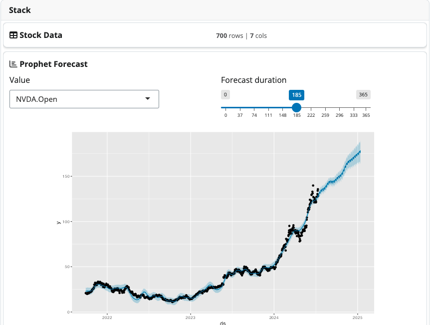

Stock model demo

2. Pharmaceutical: Clinical Trial Analysis

2.1 AE Forest Plot

This forest plot visualizes the relative risk of adverse events between two treatment arms in a clinical trial. In this case, it compares “Xanomeline High Dose” to “Xanomeline Low Dose” starting from the pharmaverseadam adae dataset. As you may notice, the new_forest_plot_block is a quite complex block. Part of the code is isolated in a function create_ae_forest_plot so that the main block constructor is more readable.

Toggle code

library(dplyr)
library(tidyr)
library(forestplot)
library(blockr.pharmaverseadam)

# Function to create adverse event forest plot
create_ae_forest_plot <- function(data, usubjid_col, arm_col, aedecod_col, n_events) {
  data <- data |> filter(.data[[arm_col]] != "Placebo")
  # Convert column names to strings
  usubjid_col <- as.character(substitute(usubjid_col))
  arm_col <- as.character(substitute(arm_col))
  aedecod_col <- as.character(substitute(aedecod_col))

  # Calculate the total number of subjects in each arm
  n_subjects <- data |>
    select(all_of(c(usubjid_col, arm_col))) |>
    distinct() |>
    group_by(across(all_of(arm_col))) |>
    summarise(n = n(), .groups = "drop")

  # Calculate AE frequencies and proportions
  ae_summary <- data |>
    group_by(across(all_of(c(arm_col, aedecod_col)))) |>
    summarise(n_events = n_distinct(.data[[usubjid_col]]), .groups = "drop") |>
    left_join(n_subjects, by = arm_col) |>
    mutate(proportion = n_events / n)

  # Select top N most frequent AEs across all arms
  top_aes <- ae_summary |>
    group_by(across(all_of(aedecod_col))) |>
    summarise(total_events = sum(n_events), .groups = "drop") |>
    top_n(n_events, total_events) |>
    pull(all_of(aedecod_col))

  # Get unique treatment arms
  arms <- unique(data[[arm_col]])
  if (length(arms) != 2) {
    stop("This plot requires exactly two treatment arms.")
  }
  active_arm <- arms[1]
  control_arm <- arms[2]

  # Filter for top AEs and calculate relative risk
  ae_rr <- ae_summary |>
    filter(.data[[aedecod_col]] %in% top_aes) |>
    pivot_wider(
      id_cols = all_of(aedecod_col),
      names_from = all_of(arm_col),
      values_from = c(n_events, n, proportion)
    ) |>
    mutate(
      RR = .data[[paste0("proportion_", active_arm)]] / .data[[paste0("proportion_", control_arm)]],
      lower_ci = exp(log(RR) - 1.96 * sqrt(
        1 / .data[[paste0("n_events_", active_arm)]] +
          1 / .data[[paste0("n_events_", control_arm)]] -
          1 / .data[[paste0("n_", active_arm)]] -
          1 / .data[[paste0("n_", control_arm)]]
      )),
      upper_ci = exp(log(RR) + 1.96 * sqrt(
        1 / .data[[paste0("n_events_", active_arm)]] +
          1 / .data[[paste0("n_events_", control_arm)]] -
          1 / .data[[paste0("n_", active_arm)]] -
          1 / .data[[paste0("n_", control_arm)]]
      ))
    )

  # Prepare data for forest plot
  forest_data <- ae_rr |>
    mutate(
      label = paste0(
        .data[[aedecod_col]], " (",
        .data[[paste0("n_events_", active_arm)]], "/", .data[[paste0("n_", active_arm)]], " vs ",
        .data[[paste0("n_events_", control_arm)]], "/", .data[[paste0("n_", control_arm)]], ")"
      )
    )

  # Create forest plot
  forestplot::forestplot(
    labeltext = cbind(
      forest_data$label,
      sprintf("%.2f (%.2f-%.2f)", forest_data$RR, forest_data$lower_ci, forest_data$upper_ci)
    ),
    mean = forest_data$RR,
    lower = forest_data$lower_ci,
    upper = forest_data$upper_ci,
    align = c("l", "r"),
    graphwidth = unit(60, "mm"),
    cex = 0.9,
    lineheight = unit(8, "mm"),
    boxsize = 0.35,
    col = fpColors(box = "royalblue", line = "darkblue", summary = "royalblue"),
    txt_gp = fpTxtGp(label = gpar(cex = 0.9), ticks = gpar(cex = 0.9), xlab = gpar(cex = 0.9)),
    xlab = paste("Relative Risk (", active_arm, " / ", control_arm, ")"),
    zero = 1,
    lwd.zero = 2,
    lwd.ci = 2,
    xticks = c(0.5, 1, 2, 4),
    grid = TRUE,
    title = paste("Relative Risk of Adverse Events (", active_arm, " vs ", control_arm, ")")
  )
}

new_forest_plot_block <- function(...) {
  new_block(
    fields = list(
      usubjid_col = new_select_field(
        "USUBJID",
        function(data) colnames(data),
        multiple = FALSE,
        title = "Subject ID Column"
      ),
      arm_col = new_select_field(
        "ACTARM",
        function(data) colnames(data),
        multiple = FALSE,
        title = "Treatment Arm Column"
      ),
      aedecod_col = new_select_field(
        "AEDECOD",
        function(data) colnames(data),
        multiple = FALSE,
        title = "AE Term Column"
      ),
      n_events = new_numeric_field(
        10,
        min = 5, max = 20, step = 1,
        title = "Number of Top AEs to Display"
      )
    ),
    expr = quote({
      create_ae_forest_plot(data, .(usubjid_col), .(arm_col), .(aedecod_col), .(n_events))
    }),
    class = c("adverse_event_plot_block", "plot_block"),
    ...
  )
}

# Register the custom block
register_block(
  new_forest_plot_block,
  name = "Adverse Event Forest Plot",
  description = "Create a forest plot of adverse events comparing two treatment arms",
  category = "plot",
  classes = c("adverse_event_plot_block", "plot_block"),
  input = "data.frame",
  output = "plot"
)

# Create the stack
clinical_trial_stack <- new_stack(
  new_adam_block(selected = "adae"),
  # filter_in_block(),
  new_forest_plot_block()
)

serve_stack(clinical_trial_stack)

2.2 Demographics Table

This demographics table is taken from the {cardinal} package of FDA Safety Tables and Figures and demonstrates gt and rtables outputs starting from the pharmaverseadam adsl dataset. As a side note, the below block requires some extra helpers to work properly which you can find here in the {blockr.cardinal} package.

library(shiny)
library(blockr)
library(cardinal)
library(blockr.pharmaverseadam)

new_cardinal02_block <- function(...) {
  all_cols <- function(data) colnames(data)

  fields <- list(
    columns = new_select_field(
      c("SEX", "AGE", "AGEGR1", "RACE", "ETHNIC", "COUNTRY"),
      all_cols,
      multiple = TRUE,
      title = "Variables"
    )
  )

  expr <- quote({
    data <- droplevels(data)

    rtables <- cardinal::make_table_02(
      df = data,
      vars = .(columns)
    )

    gt <- cardinal::make_table_02_gtsum(
      df = data,
      vars = .(columns)
    )

    list(
      rtables = rtables,
      gt = gt
    )
  })

  new_block(
    expr = expr,
    fields = fields,
    ...,
    class = c("cardinal02_block", "rtables_block", "submit_block")
  )
}

register_block(
  new_cardinal02_block,
  "Cardinal 02",
  "A Cardinal 02 table",
  category = "table",
  input = "data.frame",
  output = "list",
  classes = c("cardinal02_block", "rtables_block", "submit_block")
)


# Create the stack
rtables_stack <- new_stack(
  new_adam_block(selected = "adsl"),
  new_cardinal02_block()
)

serve_stack(rtables_stack)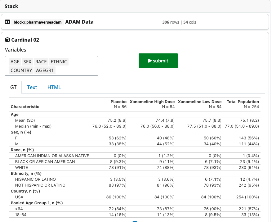

Cardinal demo

3. Environmental Science: Air Quality Analysis and Prediction

This example demonstrates a pipeline for analyzing air quality data and predicting future pollution levels using actual data from the openair package. This pipeline imports actual air quality data from the openair package and forecasts future pollution levels using an ARIMA model.

library(blockr)
library(openair)
library(forecast)

# Custom block for air quality data import
new_air_quality_block <- function(...) {
  new_block(
    fields = list(
      site = new_select_field(
        "kc1",
        \() openair::importMeta()$code,
        multiple = FALSE,
        title = "Monitoring Site"
      ),
      start_year = new_numeric_field(
        2020,
        min = 1990,
        max = as.numeric(format(Sys.Date(), "%Y")),
        step = 1,
        title = "Start Year"
      ),
      end_year = new_numeric_field(
        as.numeric(format(Sys.Date(), "%Y")),
        min = 1990,
        max = as.numeric(format(Sys.Date(), "%Y")),
        step = 1,
        title = "End Year"
      )
    ),
    expr = quote({
      importAURN(site = .(site), year = .(start_year):.(end_year)) |> tail(700)
    }),
    class = c("air_quality_block", "data_block"),
    ...
  )
}


# Custom block for pollution forecasting
new_pollution_forecast_block <- function(columns = character(), ...) {
  all_cols <- function(data) setdiff(colnames(data), c("date", "site", "source"))

  new_block(
    fields = list(
      pollutant = new_select_field(columns, all_cols, multiple = FALSE, title = "Pollutant"),
      horizon = new_slider_field(
        30,
        min = 1,
        max = 365,
        step = 1,
        title = "Forecast Horizon (days)"
      )
    ),
    expr = quote({
      ts_data <- ts(na.omit(data[[.(pollutant)]]), frequency = 365)
      model <- auto.arima(ts_data)
      forecast_result <- forecast(model, h = .(horizon))
      plot(forecast_result, main = paste("Forecast of", .(pollutant), "levels"))
    }),
    class = c("pollution_forecast_block", "plot_block"),
    ...
  )
}

# Register custom blocks
register_block(
  new_air_quality_block,
  name = "Air Quality Data",
  description = "Import air quality data",
  category = "data",
  classes = c("air_quality_block", "data_block"),
  input = NA_character_,
  output = "data.frame"
)

register_block(
  new_pollution_forecast_block,
  name = "Pollution Forecast",
  description = "Forecast pollution levels",
  category = "plot",
  classes = c("pollution_forecast_block", "plot_block"),
  input = "data.frame",
  output = "plot"
)

# Create the stack
air_quality_stack <- new_stack(
  new_air_quality_block(),
  new_pollution_forecast_block(columns = "no2")
)

serve_stack(air_quality_stack)

4. Marketing: Causal Impact Analysis of Marketing Interventions

This example demonstrates how to use CausalImpact to analyze the effect of marketing interventions on sales data. This pipeline generates dummy marketing data with an intervention, then uses CausalImpact to analyze the effect of the intervention on sales. This requires to define a new date field as shown below.

library(shiny)
new_date_field <- function(value = Sys.Date(), min = NULL, max = NULL, ...) {
  blockr::new_field(
    value = value,
    min = min,
    max = max,
    ...,
    class = "date_field"
  )
}

date_field <- function(...) {
  validate_field(new_date_field(...))
}

#' @method ui_input date_field
#' @export
ui_input.date_field <- function(x, id, name) {
  shiny::dateInput(
    blockr::input_ids(x, id),
    name,
    value = blockr::value(x, "value"),
    min = blockr::value(x, "min"),
    max = blockr::value(x, "max")
  )
}

#' @method validate_field date_field
#' @export
validate_field.date_field <- function(x, ...) {
  x
}

#' @method ui_update date_field
#' @export
ui_update.date_field <- function(x, session, id, name) {
  updateDateInput(
    session,
    blockr::input_ids(x, id),
    blockr::get_field_name(x, name),
    value = blockr::value(x),
    min = blockr::value(x, "min"),
    max = blockr::value(x, "max")
  )
}

library(blockr)
library(CausalImpact)
library(dplyr)

# Custom block to load and prepare marketing data
new_marketing_data_block <- function(...) {
  new_block(
    fields = list(
      start_date = date_field(
        Sys.Date() - 365,
        min = Sys.Date() - 730,
        max = Sys.Date() - 1,
        label = "Start Date"
      ),
      intervention_date = date_field(
        Sys.Date() - 180,
        min = Sys.Date() - 729,
        max = Sys.Date(),
        label = "Intervention Date"
      ),
      end_date = date_field(
        Sys.Date(),
        min = Sys.Date() - 364,
        max = Sys.Date(),
        label = "End Date"
      )
    ),
    expr = quote({
      # Generate dummy data for demonstration
      dates <- seq(as.Date(.(start_date)), as.Date(.(end_date)), by = "day")
      sales <- cumsum(rnorm(length(dates), mean = 100, sd = 10))
      ad_spend <- cumsum(rnorm(length(dates), mean = 50, sd = 5))

      # Add intervention effect
      intervention_index <- which(dates == as.Date(.(intervention_date)))
      sales[intervention_index:length(sales)] <- sales[intervention_index:length(sales)] * 1.2

      data.frame(
        date = dates,
        sales = sales,
        ad_spend = ad_spend
      )
    }),
    class = c("marketing_data_block", "data_block"),
    ...
  )
}

# Custom block for CausalImpact analysis
new_causal_impact_block <- function(columns = character(), ...) {
  all_cols <- function(data) colnames(data)[2:length(colnames(data))]

  new_block(
    fields = list(
      response_var = new_select_field(
        columns,
        all_cols,
        multiple = FALSE,
        title = "Response Variable"
      ),
      covariate_var = new_select_field(
        columns,
        all_cols,
        multiple = FALSE,
        title = "Covariate Variable"
      ),
      pre_period_end = date_field(
        Sys.Date() - 181,
        min = Sys.Date() - 729,
        max = Sys.Date() - 1,
        label = "Pre-Period End Date"
      ),
      post_period_start = date_field(
        Sys.Date() - 180,
        min = Sys.Date() - 728,
        max = Sys.Date(),
        label = "Post-Period Start Date"
      )
    ),
    expr = quote({
      data <- data.frame(
        date = data$date,
        y = data[[.(response_var)]],
        x = data[[.(covariate_var)]]
      )
      pre_period <- c(min(as.Date(data$date)), as.Date(.(pre_period_end)))
      post_period <- c(as.Date(.(post_period_start)), max(as.Date(data$date)))

      impact <- CausalImpact(data, pre_period, post_period)
      plot(impact)
    }),
    class = c("causal_impact_block", "plot_block"),
    ...
  )
}

# Register custom blocks
register_block(
  new_marketing_data_block,
  name = "Marketing Data",
  description = "Load and prepare marketing data",
  category = "data",
  classes = c("marketing_data_block", "data_block"),
  input = NA_character_,
  output = "data.frame"
)
register_block(
  new_causal_impact_block,
  name = "Causal Impact Analysis",
  description = "Perform Causal Impact analysis on marketing data",
  category = "plot",
  classes = c("causal_impact_block", "plot_block"),
  input = "data.frame",
  output = "plot"
)

# Create the stack
marketing_impact_stack <- new_stack(
  new_marketing_data_block(),
  new_causal_impact_block()
)

serve_stack(marketing_impact_stack)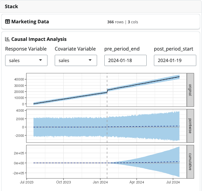

Marketing demo

5. Dynamical systems

In the below example, we implemented the Lorenz attractor and solve it with the {pracma} R package (technically, the reason using {pracma} over deSolve or diffeqr is because only {pracma} is available for shinylive required by the embeded demo).

Toggle code

library(blockr)
library(pracma)
library(blockr.ggplot2)

new_ode_block <- function(...) {

  lorenz <- function (t, y, parms) {
    c(
      X = parms[1] * y[1] + y[2] * y[3],
      Y = parms[2] * (y[2] - y[3]),
      Z = -y[1] * y[2] + parms[3] * y[2] - y[3]
    )
  }

  fields <- list(
    a = new_numeric_field(-8/3, -10, 20),
    b = new_numeric_field(-10, -50, 100),
    c = new_numeric_field(28, 1, 100)
  )

  new_block(
    fields = fields,
    expr = substitute(
      as.data.frame(
        ode45(
          fun, 
          y0 = c(X = 1, Y = 1, Z = 1),
          t0 = 0,
          tfinal = 100,
          parms = c(.(a), .(b), .(c))
        )
      ),
      list(fun = lorenz)
    ),
    ...,
    class = c("ode_block", "data_block")
  )
}

stack <- new_stack(
  new_ode_block,
  # Coming from blockr.ggplot2
  new_ggplot_block(
    func = c("x", "y"), 
    default_columns = c("y.1", "y.2")
  ), 
  new_geompoint_block
)
serve_stack(stack)