Build your first app
This tutorial will get you started with blockr in just a few minutes. By the end, you will have built your first data pipeline.
Start blockr
Live playground
The simplest way to try blockr is for free in our live playground at blockr.cloud. Note, you will not be able to save and restore sessions this way.
Local installation
Run the following commands to install blockr locally and then spin up an empty app:
install.packages("blockr") # Download blockr. This only needs to be run once.
blockr::run_app() # Start an empty app. Run this each time you want to boot up blockr.Installing blockr locally assumes you already have R installed on your system and are comfortable running basic R commands.
First steps
Load some data
Each empty blockr app starts with a blank canvas:
![]()
To build a workflow, simply add some blocks to your canvas, connect them, and then watch blockr automatically run the workflows!
Let’s start by adding some data. Right-click the canvas then click “Add block”:
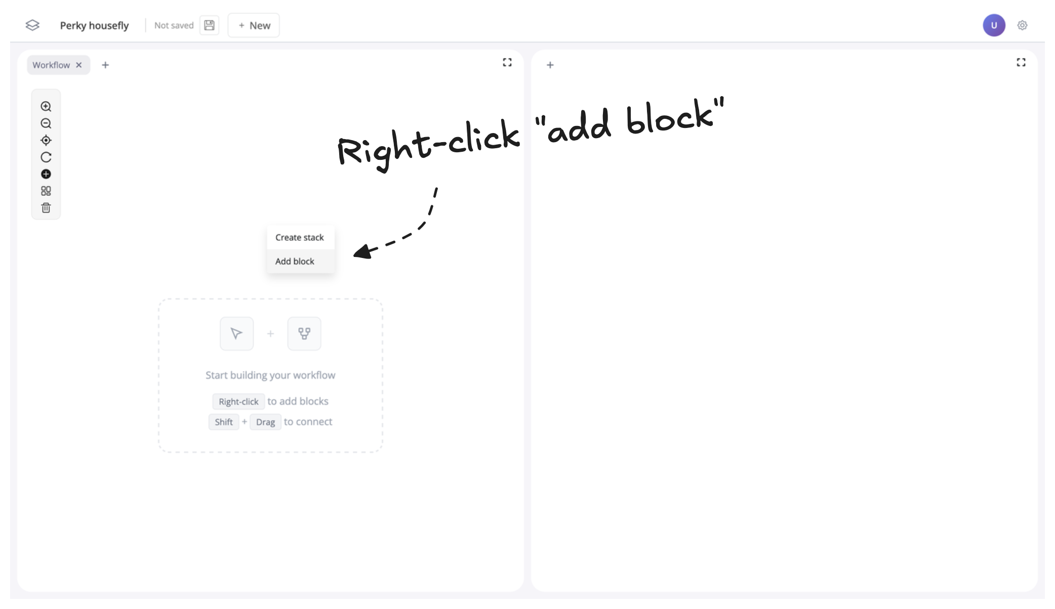
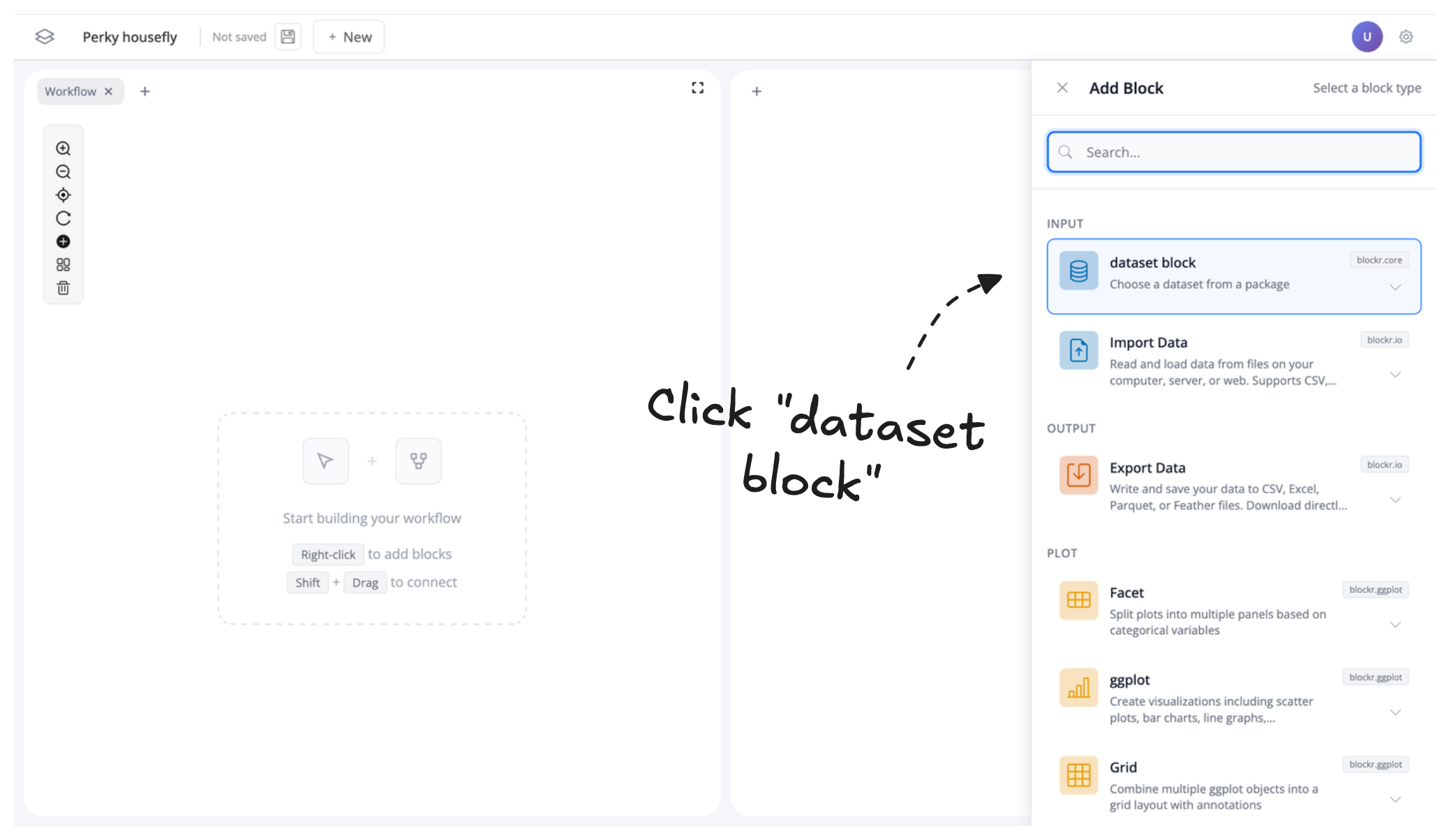
This opens the right sidebar with a block selection menu. Here, blocks are sorted into categories like Inputs, Outputs, and Plots, so you can easily browse and discover them. You can also use the search bar to find blocks.
For now, let’s click “dataset block” to load an example data block, preconfigured with a bunch of different datasets.
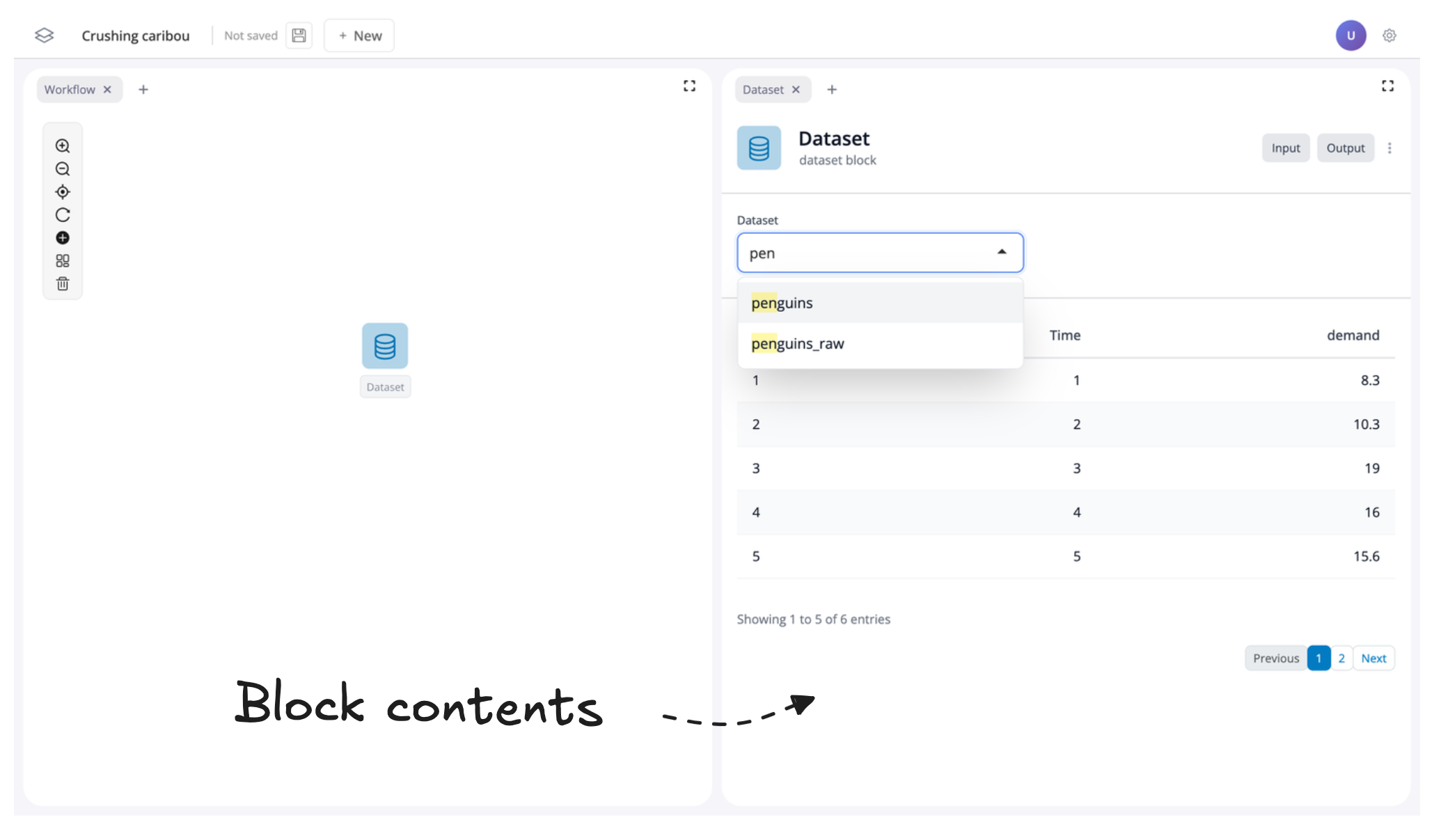
Once the block is added to the canvas, the contents of the block will be loaded to the right-hand panel. Let’s change the dataset to penguins by clicking and searching in the drop-down menu:
Filter some data
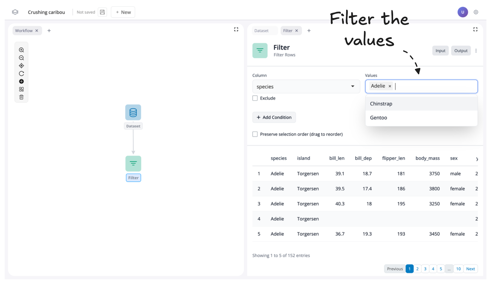
Next, let’s filter our penguins data to only return the species “Adelie” and “Chinstrap”.
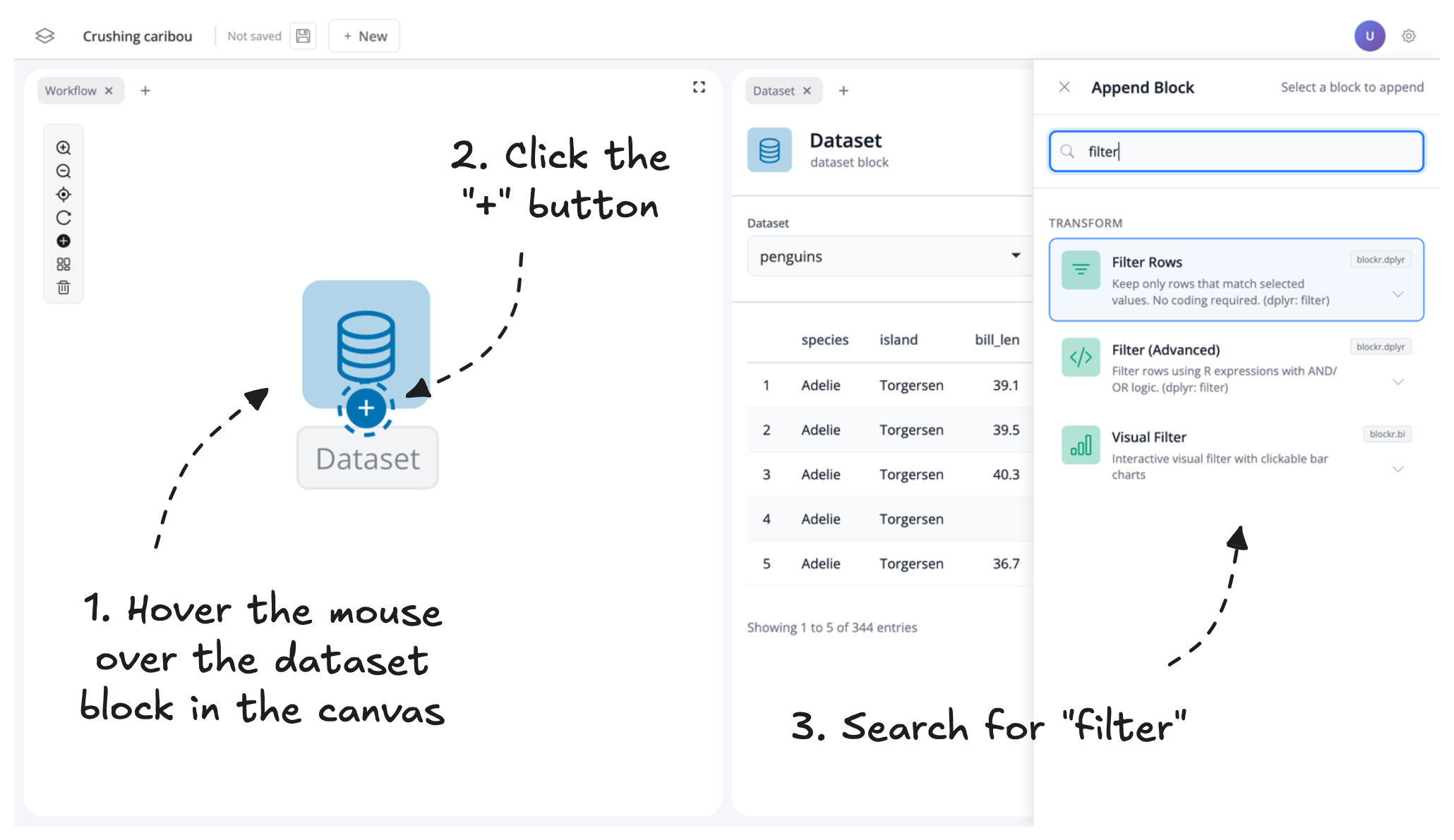
To connect a filter block:
- Hover the mouse over the dataset block
- Click the “+” button at the bottom of the block, called a port, to bring up the block menu sidebar once more:
- Search for “filter” and click “Filter Rows”
This will add a new connected filter block to the canvas. From here, we can filter the data to just keep the “Adelie” and “Chinstrap” species of penguins by seleting their values from the “Values” drop-down box:
Visualise some data
Finally, let’s finish our first pipeline by visualising some data. To do that, let’s add a visualisation block, but use a different method to do that.
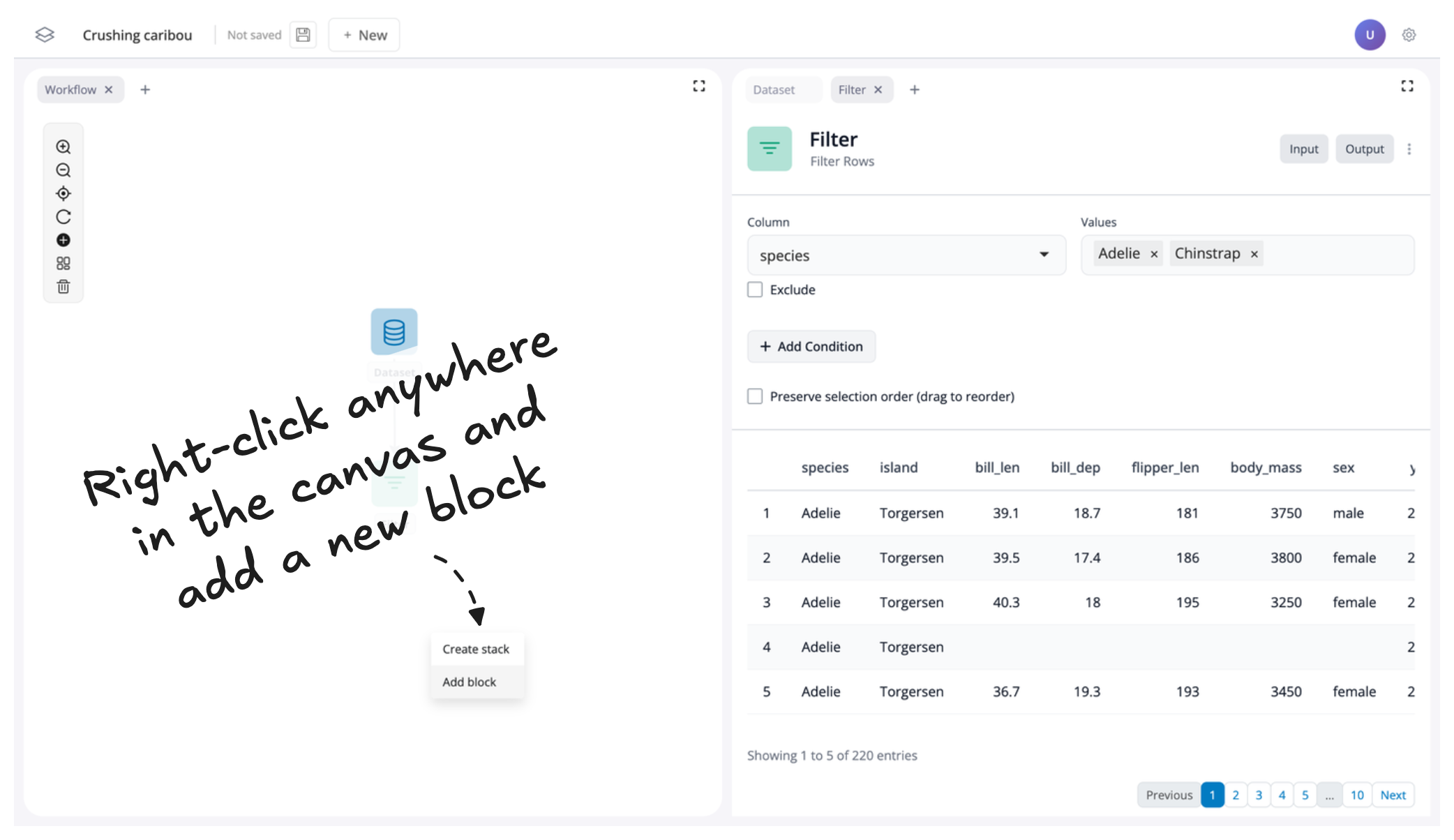
First, right-click anywhere in the canvas and click “Add block” like we did in the first step of this tutorial:
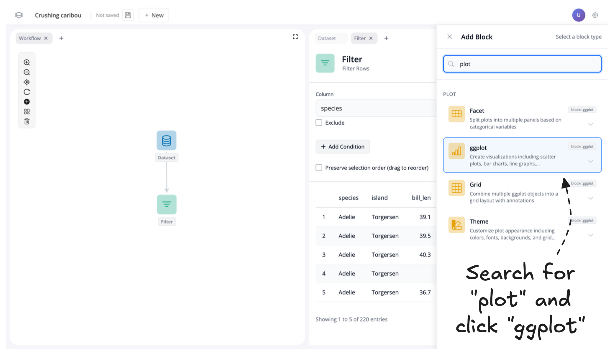
Then search for “plot” and click “ggplot” to add a plot block to our canvas:
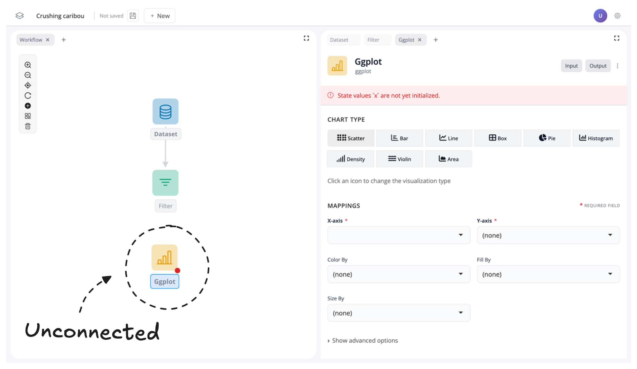
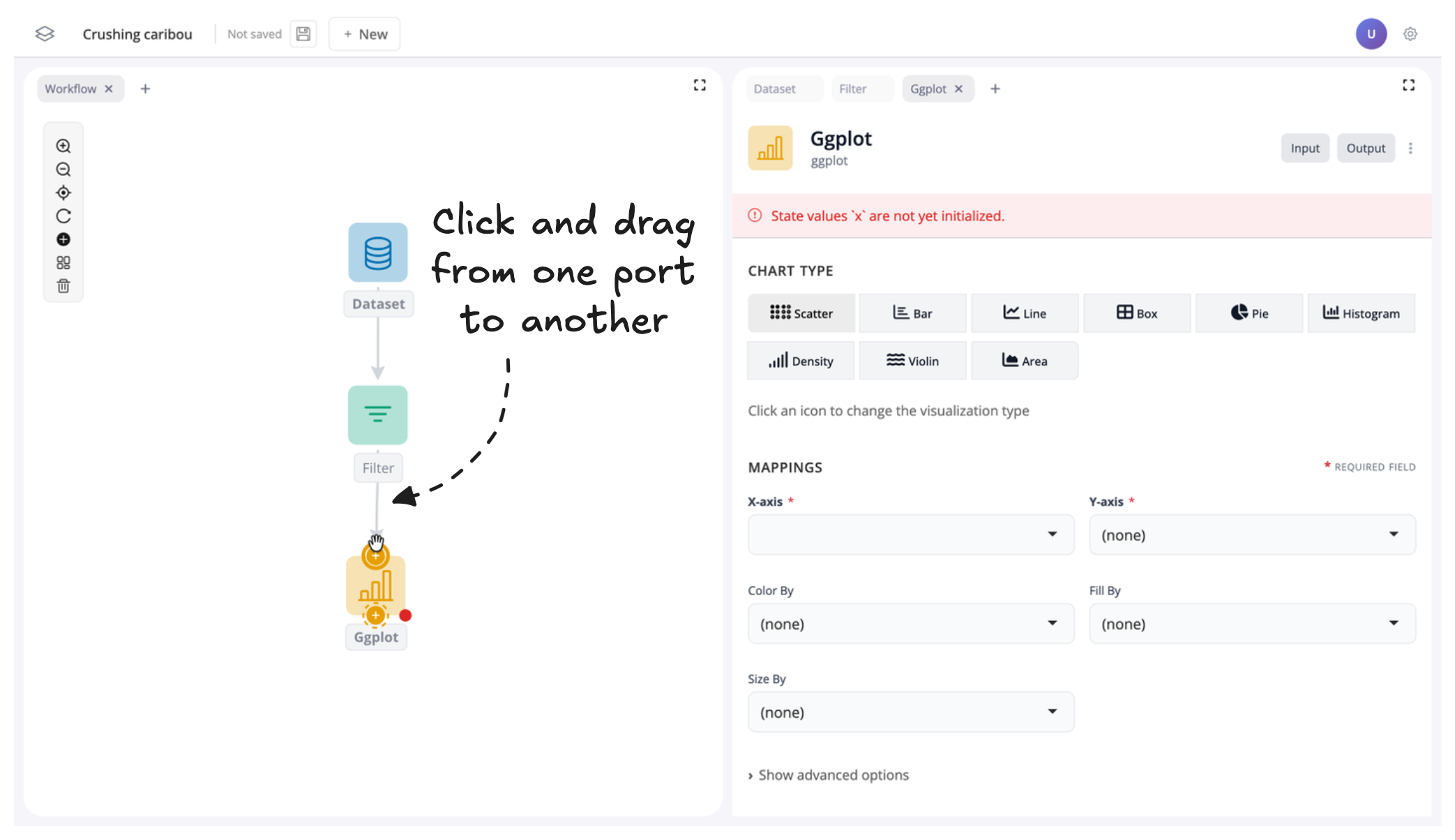
This will add an unconnected plot block to our canvas. We know that the block is unconnected because there are no connecting arrows from our other blocks to our plot block:
To connect the plot block, hover the mouse over the filter block to view the available ports. Then, click and drag from the port on the bottom of the filter block to the port on the top of the plot block.
Notice how the dotted line around the port on the plot block becomes solid to indicate that a connection can be made.
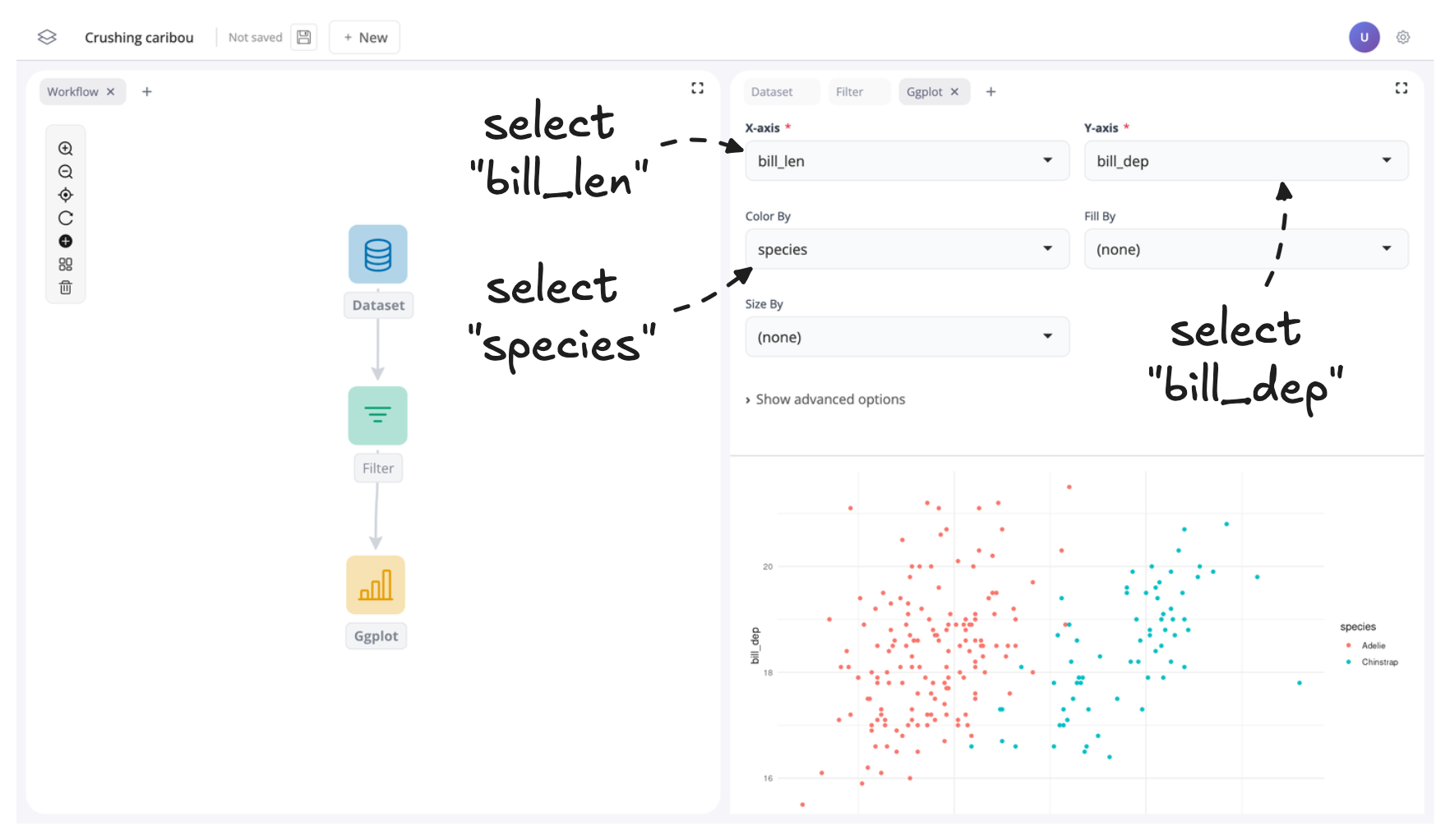
To finish let’s populate some of the inputs in the plot block to create a scatter plot of penguin bill length versus bill depth across the different species:
Summary
And that’s it! You’ve learned how to add blocks to the canvas, search for blocks, and connect them using ports. You now have the skills to import, transform, and visualize data in blockr.